Particle Swarm Optimization

This post is about a single objective particle swarm optimization algorithm. Particle Swarm Optimization is a nature-inspired heuristic optimization algorithm. A resource for psuedo-code for this algorithm can be found here. This is one of several types of heuristic optimization algorithms that allow one to find the global minimum of a function subject to any constraints without calculating any gradients.

Single objective optimization consists of finding the global miniumum of a function, \(f(x, y)\), over a range of bounds for x and y, and subject to some constraint. For example, consider the function:

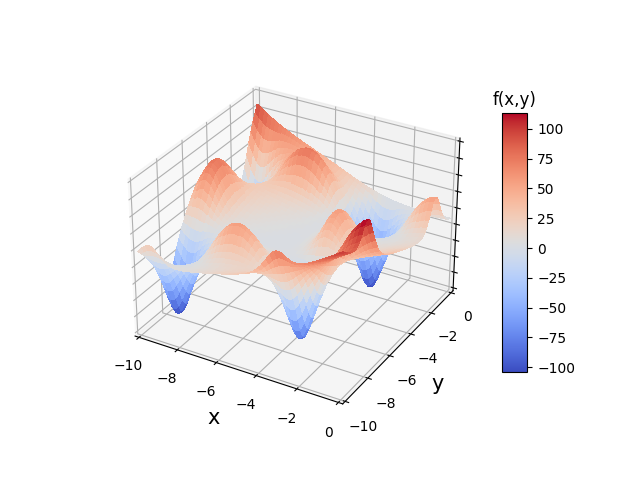
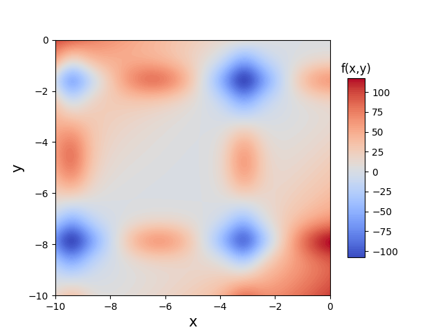
The goal of Single Objective Optimization is to find the global minimum of this function, which is \(f(-3.13, -1.58) = -106.76\). However, this function has multiple local minumums, which can make it difficult to solve. A top-view contour plot of this function is also shown below.

There are two main classes of optimization algorithms:

• Gradient-based Algorithms: Calculates the local gradients of the function and moves towards the negative values
• Heuristic Algorithms: Designed to solve problems quickly, often attempting to imitate nature.

Particle swarm optimization (PSO) is an heuristic algorithm designed to simulate social behavior, or swarm intelligence. In order to find the global minimum, a swarm of particles is created and placed in the search space. Then, each particle is given velocity its p, moving it towards its personal best position and the global best position.

Each iteration, every particle in the swarm moves while updting the global and personal best positions in search of the global minimum. If a particle moves to a location outside of the search space, then the particles position is set to the boundary of the space. If there are constraints on the problem, then any particle violating those constraints are considered as inelegible to become one of the ‘best’ positions. The stopping condition is defined when either the global best position does not change for a number of iterations, or the maximum number of iterations is exceeded.

Particles

In order for the algorithm to work, particles need to be able keep track of their own data, send data, recieve data, and move. For this, we will make a particle class.

1
2
3
4
5
6
7
8
9
10
11
class Particle():
    def __init__(self, func, constraintfunc, position, LB, UB):
        self.func = func
        self.constraintfunc = constraintfunc
        self.x_current = position
        self.v_current = np.zeros_like(position)
        self.f_current, self.eligible = self.evaluate(position)
        self.fp_best = self.f_current
        self.xp_best = np.zeros_like(position)
        self.LB = LB
        self.UB = UB

When initializing a particle, two functions are passed. The first is the function to be minimized, taking in an array of input variables and returns the value. The second is a constraint function that takes in the array of input variables and the function value returning a boolean that states whether or not the position is feasible. An initial position is also given, as well as the upper and lower bounds on the input variables. The initial position is then evaluated, and the intial velocity is set to zero. The personal best position and value are set as the intial.

The evaluation function takes a position, evaluates it to get the function value, then determines whether or not the position is within the constraints.

1
2
3
4
    def evaluate(self, x):
        f_vals = self.func(x)
        eligible = self.constraintfunc(f_vals, x)
        return f_vals, eligible

Now, we must give the particles a way to move. We want the paricles to move towards the global minimum. To do this, we will use the following formula.

In this equation rand() is a randomly generated number between 0 and 1. \(\alpha\) is a parameter between 0 and 1 that determines the weighting of the previous velocity in the new velocity. Then, we have the hyperparameters A and B, determining the weighting of the particles personal best and the swarms global best position. These parameters have a large effect on performance, but the suggested range is between 1 and 3. They will be set as inputs to the move function, defined below.

1
2
3
4
5
6
7
8
9
10
11
12
13
14
15
16
17
    def Move(self, xg_best, alpha, A, B):
        Vi = (alpha*self.v_current
             + A*np.random.rand()*(self.xp_best - self.x_current)
             + B*np.random.rand()*(xg_best - self.x_current))
        self.x_current = self.x_current + Vi
        # Check for new positions outside of the bounds
        for variable in range(len(self.x_current)):
            if self.x_current[variable] < self.LB[variable]:
                self.x_current[variable] = self.LB[variable]
            if self.x_current[variable] > self.UB[variable]:
                self.x_current[variable] = self.UB[variable]
        # re-evaluate functions
        self.f_current, self.eligible = self.evaluate(self.x_current)
        if self.eligible:
            if self.f_current < self.fp_best:
                self.fp_best = self.f_current
                self.xp_best = self.x_current

The Swarm

Now, a function created to build the swarm.

1
2
3
4
5
6
7
8
9
10
11
def pso(efunc, cfunc, ipop, LB, UB, Nmx, alpha, A, B):
    pop = np.empty((len(ipop)), dtype=object)
    for i in range(len(ipop)):
        pop[i] = Particle(efunc, cfunc, ipop[i], LB, UB)
    fg_best = 1E15
    xg_best = None
    for particle in pop:
        f_local, x_local = particle.get_best()
        if f_local < fg_best:
            fg_best = f_local
            xg_best = x_local

This function takes the evaluation and constraint functions, an initial population of position values, position upper and lower bounds, a maximum number of iterations, and finally the three hyperparameters. The first thing to happen is to take the initial positions and create the swarm of particles. Then, the swarm of particles is checked for a global best position.

Now, a counter variable fg_best_changeITER will be defined to determine how many iterations it has been since the global best value has changed. Then the loop through the iterations will begin.

1
2
3
4
5
6
7
8
9
10
11
12
13
14
15
16
17
18
19
20
21
22
	fg_best_changeITER = 0
    print('initialized')
    N = 0
    while N < Nmx:
        if N % 100 == 0:
            print('Iteration #', N)
        for particle in pop:
            particle.Move(xg_best, alpha, A, B)
        fg_best_prev = fg_best
        for particle in pop:
            f_local, x_local = particle.get_best()
            if (f_local < fg_best) and particle.elig():
                fg_best = f_local
                xg_best = x_local
        if fg_best == fg_best_prev:
            fg_best_changeITER += 1
        else:
            fg_best_changeITER = 0
        if fg_best_changeITER > 20:
            print('STOP: Best function evaluation did not change for 10 iterations')
            break
        N += 1

For each iteration the first thing that happens is the particles are moved. Then, each particle is checked against the global best, and the global best is updated. Finally, there is a check to see if the global best has changed that iteration. If it hasn’t changed for 20 iterations, then convergence is assumed and the loop ends. The function then ends by returning the number of iterations and the resulting global best position and value.

Now we can run the function, and see the results.

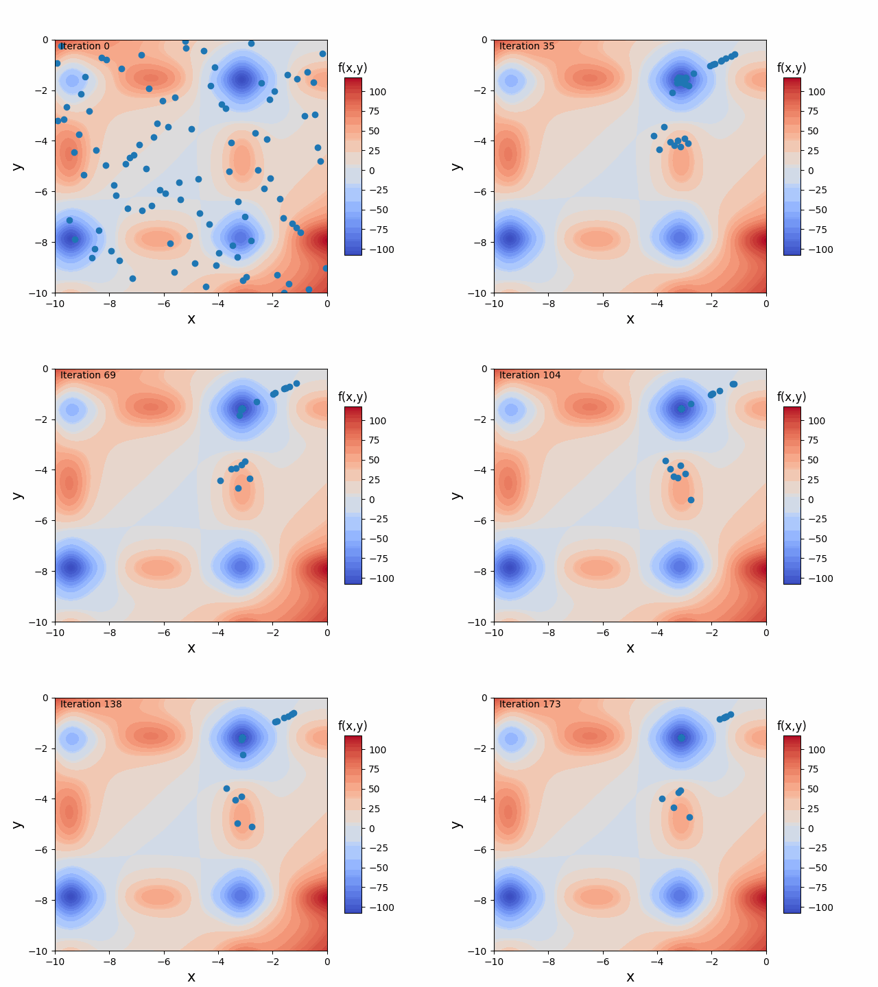
This gif shows the population’s positions at every itertion. The algorithm begins to converge very quickly, but does not stop until it is sure that the minimum will not change. several points end up moving back and forth, torn between the global best position and it’s own best position.

The code for this algorithm can be found at This Github Repository